In-Class Exercise 8 - Network Graph

Published

March 16, 2024

Modified

March 16, 2024

Loading R Packages

pacman::p_load(igraph, tidygraph, ggraph, 
               visNetwork, lubridate, clock,
               tidyverse, graphlayouts)

Loading data set

GAStech_nodes <- read_csv("data/GAStech_email_node.csv")
GAStech_edges <- read_csv("data/GAStech_email_edge-v2.csv")

GAStech_edges <- GAStech_edges %>%
  mutate(SendDate = dmy(SentDate)) %>%
  mutate(Weekday = wday(SentDate,
                        label = TRUE,
                        abbr = FALSE))

GAStech_edges_aggregated <- GAStech_edges %>%
  filter(MainSubject == "Work related") %>%
  group_by(source, target, Weekday) %>%
    summarise(Weight = n()) %>%
  filter(source!=target) %>%
  filter(Weight > 1) %>%
  ungroup()

GAStech_graph <- tbl_graph(nodes = GAStech_nodes, 
                           edges = GAStech_edges_aggregated, 
                           directed = TRUE)

GAStech_graph

# A tbl_graph: 54 nodes and 1372 edges
#
# A directed multigraph with 1 component
#
# Node Data: 54 × 4 (active)
      id label               Department     Title                               
   <dbl> <chr>               <chr>          <chr>                               
 1     1 Mat.Bramar          Administration Assistant to CEO                    
 2     2 Anda.Ribera         Administration Assistant to CFO                    
 3     3 Rachel.Pantanal     Administration Assistant to CIO                    
 4     4 Linda.Lagos         Administration Assistant to COO                    
 5     5 Ruscella.Mies.Haber Administration Assistant to Engineering Group Mana…
 6     6 Carla.Forluniau     Administration Assistant to IT Group Manager       
 7     7 Cornelia.Lais       Administration Assistant to Security Group Manager 
 8    44 Kanon.Herrero       Security       Badging Office                      
 9    45 Varja.Lagos         Security       Badging Office                      
10    46 Stenig.Fusil        Security       Building Control                    
# ℹ 44 more rows
#
# Edge Data: 1,372 × 4
   from    to Weekday Weight
  <int> <int> <ord>    <int>
1     1     2 Sunday       5
2     1     2 Monday       2
3     1     2 Tuesday      3
# ℹ 1,369 more rows

Plotting Network Graphs

Basic Network Graph

The code chunk below uses ggraph(), geom-edge_link() and geom_node_point() to plot a network graph by using GAStech_graph.

ggraph(GAStech_graph) +
  geom_edge_link() +
  geom_node_point()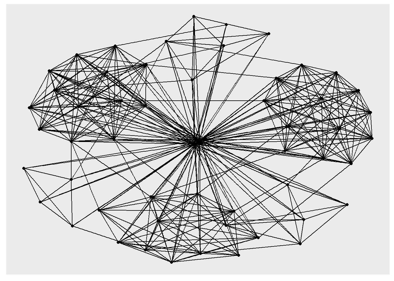

Fruchterman and Reingold Layout

The code chunks below will be used to plot the network graph using Fruchterman and Reingold layout.

g <- ggraph(GAStech_graph,
            layout = "fr") + 
  geom_edge_link(aes()) +
  geom_node_point(aes())

g + theme_graph()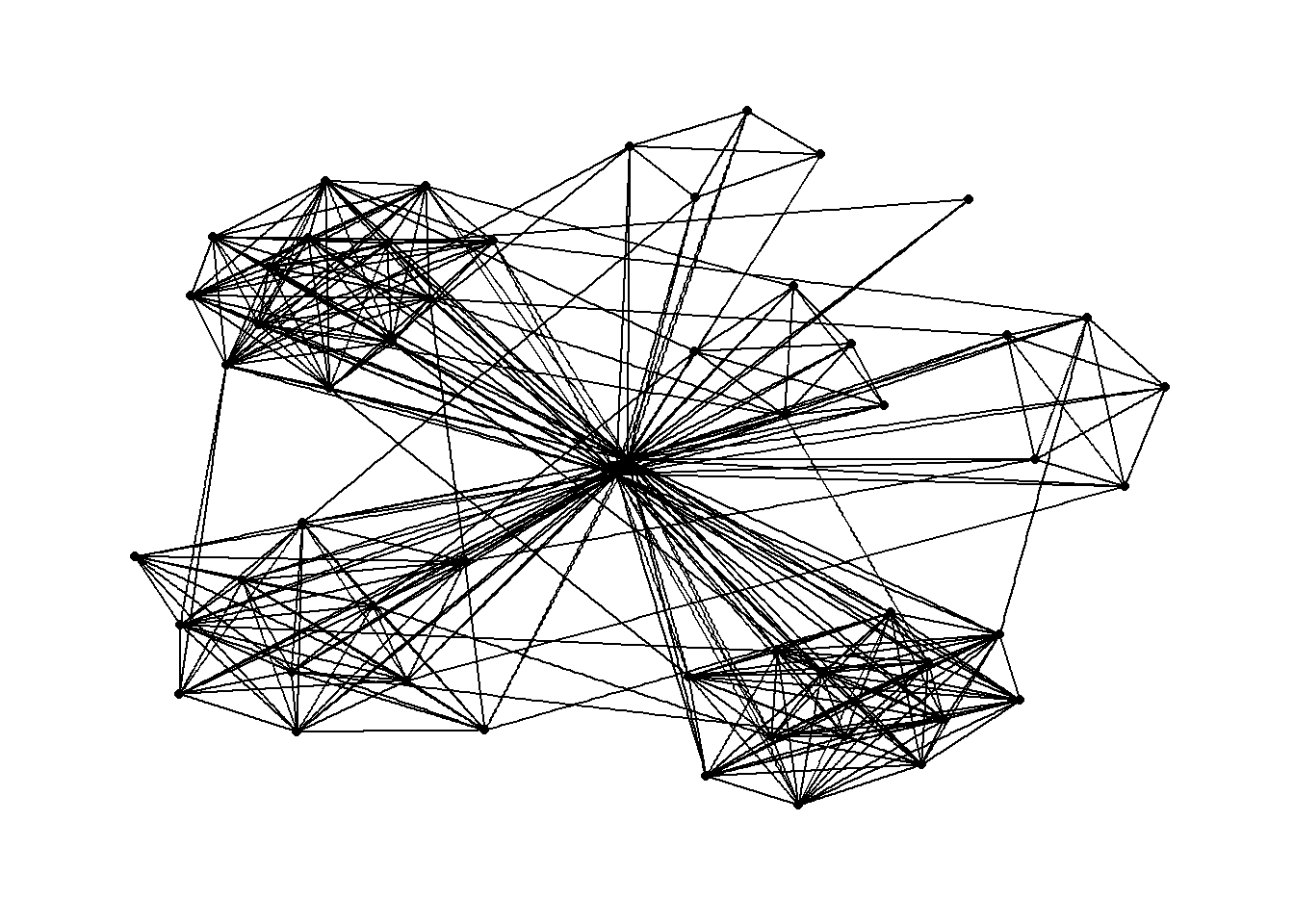

g <- ggraph(GAStech_graph,
            layout = "kk") + 
  geom_edge_link(aes()) +
  geom_node_point(aes())

g + theme_graph()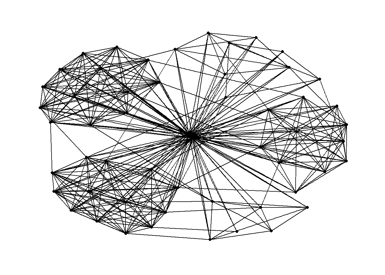

Modifying Network Nodes

In this section, we will colour each node by referring to their respective departments.

g <- ggraph(GAStech_graph, 
            layout = "nicely") + 
  geom_edge_link(aes()) +
  geom_node_point(aes(colour = Department, 
                      size = 3))

g + theme_graph()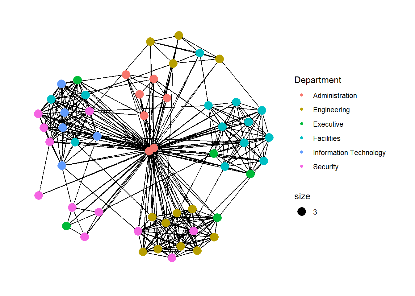

Modifying Edges

In the code chunk below, the thickness of the edges will be mapped with the Weight variable.

g <- ggraph(GAStech_graph, 
            layout = "nicely") +
  geom_edge_link(aes(width=Weight), 
                 alpha=0.2) +
  scale_edge_width(range = c(0.1, 5)) +
  geom_node_point(aes(colour = Department), 
                  size = 3)

g + theme_graph()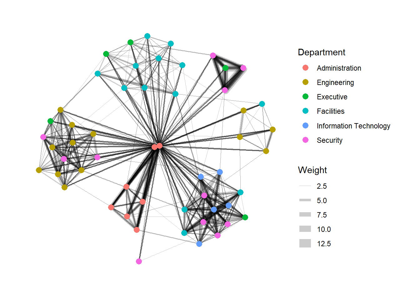

Working with `facet_edges()`

In the code chunk below, facet_edges() is used.

set_graph_style()

g <- ggraph(GAStech_graph, 
            layout = "nicely") + 
  geom_edge_link(aes(width=Weight), 
                 alpha=0.2) +
  scale_edge_width(range = c(0.1, 5)) +
  geom_node_point(aes(colour = Department), 
                  size = 2)

g + facet_edges(~Weekday)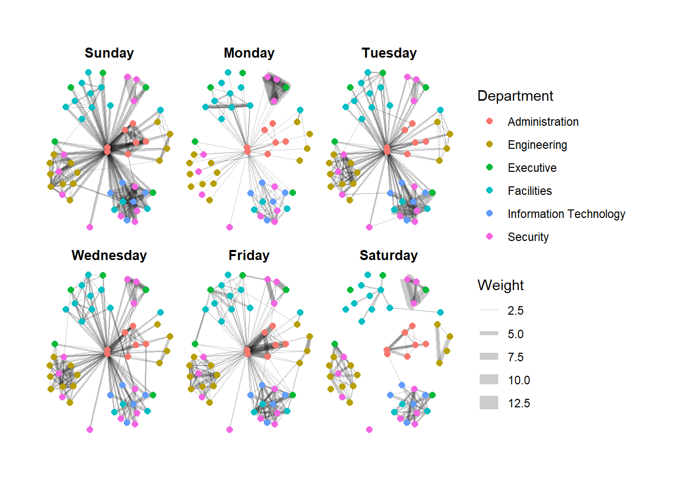

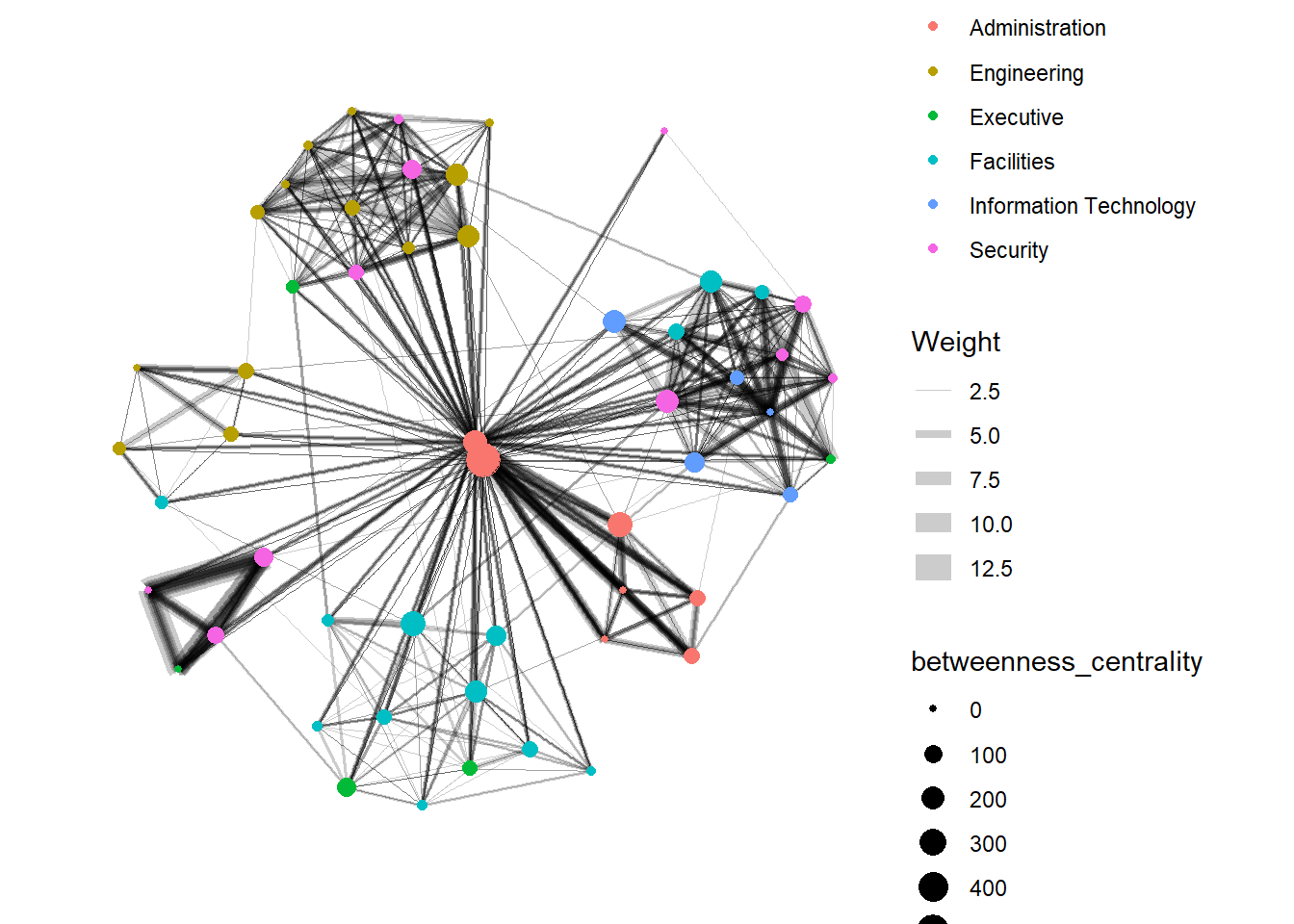
Computing Centrality Indices

g <- GAStech_graph %>%
  mutate(betweenness_centrality = centrality_betweenness()) %>%
  ggraph(layout = "fr") + 
  geom_edge_link(aes(width=Weight), 
                 alpha=0.2) +
  scale_edge_width(range = c(0.1, 5)) +
  geom_node_point(aes(colour = Department,
            size=betweenness_centrality))
g + theme_graph()