pacman::p_load(tidyverse, dplyr, tidyr,
               sf, lubridate,plotly,
tmap, spdep, sfdep, knitr, forcats)Take-home Exercise 4d - plotting for project poster
Getting Started
Loading R packages and Data prep
ACLED_MMR <- read_csv("data/MMR.csv")mmr_shp_mimu_2 <- st_read(dsn = "data/geospatial3",
layer = "mmr_polbnda_adm2_250k_mimu")Reading layer `mmr_polbnda_adm2_250k_mimu' from data source
`C:\imranmi\ISSS608-VAA\Take-home-ex\Take-home-Ex4d\data\geospatial3'
using driver `ESRI Shapefile'
Simple feature collection with 80 features and 7 fields
Geometry type: MULTIPOLYGON
Dimension: XY
Bounding box: xmin: 92.1721 ymin: 9.696844 xmax: 101.17 ymax: 28.54554
Geodetic CRS: WGS 84ACLED_MMR_1 <- ACLED_MMR %>%
mutate(admin1 = case_when(
admin1 == "Bago-East" ~ "Bago (East)",
admin1 == "Bago-West" ~ "Bago (West)",
admin1 == "Shan-North" ~ "Shan (North)",
admin1 == "Shan-South" ~ "Shan (South)",
admin1 == "Shan-East" ~ "Shan (East)",
TRUE ~ as.character(admin1)
))ACLED_MMR_1 <- ACLED_MMR_1 %>%
mutate(admin2 = case_when(
admin2 == "Yangon-East" ~ "Yangon (East)",
admin2 == "Yangon-West" ~ "Yangon (West)",
admin2 == "Yangon-North" ~ "Yangon (North)",
admin2 == "Yangon-South" ~ "Yangon (South)",
admin2 == "Mong Pawk (Wa SAD)" ~ "Tachileik",
admin2 == "Nay Pyi Taw" ~ "Det Khi Na",
admin2 == "Yangon" ~ "Yangon (West)",
TRUE ~ as.character(admin2)
))Loading in previously wrangled data for quarterly data
Events_2 <- read_csv("data/df_complete.csv")Events_admin2 <- left_join(mmr_shp_mimu_2, Events_2,
by = c("DT" = "admin2"))Events_admin2 <- Events_admin2 %>%
select(-OBJECTID, -ST, -ST_PCODE,
-DT_PCODE, -DT_MMR, -PCode_V)class(Events_admin2)[1] "sf" "data.frame"Filtering for Event type == Battles, for all quarters from 2021-2023
Show the code
Battles2021Q1 <- Events_admin2 %>%
  filter(quarter == "2021Q1", event_type == "Battles")

Battles2021Q2 <- Events_admin2 %>%
  filter(quarter == "2021Q2", event_type == "Battles")

Battles2021Q3 <- Events_admin2 %>%
  filter(quarter == "2021Q3", event_type == "Battles")

Battles2021Q4 <- Events_admin2 %>%
  filter(quarter == "2021Q4", event_type == "Battles")

Battles2022Q1 <- Events_admin2 %>%
  filter(quarter == "2022Q1", event_type == "Battles")

Battles2022Q2 <- Events_admin2 %>%
  filter(quarter == "2022Q2", event_type == "Battles")

Battles2022Q3 <- Events_admin2 %>%
  filter(quarter == "2022Q3", event_type == "Battles")

Battles2022Q4 <- Events_admin2 %>%
  filter(quarter == "2022Q4", event_type == "Battles")

Battles2023Q1 <- Events_admin2 %>%
  filter(quarter == "2023Q1", event_type == "Battles")

Battles2023Q2 <- Events_admin2 %>%
  filter(quarter == "2023Q2", event_type == "Battles")

Battles2023Q3 <- Events_admin2 %>%
  filter(quarter == "2023Q3", event_type == "Battles")

Battles2023Q4 <- Events_admin2 %>%
  filter(quarter == "2023Q4", event_type == "Battles")
Deriving contiguity weights: Queen’s method
Show the code
wm_q1 <- Battles2021Q1 %>%
  mutate(nb = st_contiguity(geometry),
         wt = st_weights(nb,
                         style = "W"),
         .before = 1)

wm_q2 <- Battles2021Q2 %>%
  mutate(nb = st_contiguity(geometry),
         wt = st_weights(nb,
                         style = "W"),
         .before = 1)

wm_q3 <- Battles2021Q3 %>%
  mutate(nb = st_contiguity(geometry),
         wt = st_weights(nb,
                         style = "W"),
         .before = 1)

wm_q4 <- Battles2021Q4 %>%
  mutate(nb = st_contiguity(geometry),
         wt = st_weights(nb,
                         style = "W"),
         .before = 1)

wm_q5 <- Battles2022Q1 %>%
  mutate(nb = st_contiguity(geometry),
         wt = st_weights(nb,
                         style = "W"),
         .before = 1)

wm_q6 <- Battles2022Q2 %>%
  mutate(nb = st_contiguity(geometry),
         wt = st_weights(nb,
                         style = "W"),
         .before = 1)

wm_q7 <- Battles2022Q3 %>%
  mutate(nb = st_contiguity(geometry),
         wt = st_weights(nb,
                         style = "W"),
         .before = 1)

wm_q8 <- Battles2022Q4 %>%
  mutate(nb = st_contiguity(geometry),
         wt = st_weights(nb,
                         style = "W"),
         .before = 1)

wm_q9 <- Battles2023Q1 %>%
  mutate(nb = st_contiguity(geometry),
         wt = st_weights(nb,
                         style = "W"),
         .before = 1)

wm_q10 <- Battles2023Q2 %>%
  mutate(nb = st_contiguity(geometry),
         wt = st_weights(nb,
                         style = "W"),
         .before = 1)

wm_q11 <- Battles2023Q3 %>%
  mutate(nb = st_contiguity(geometry),
         wt = st_weights(nb,
                         style = "W"),
         .before = 1)

wm_q12 <- Battles2023Q4 %>%
  mutate(nb = st_contiguity(geometry),
         wt = st_weights(nb,
                         style = "W"),
         .before = 1)
No of sims = 199
Show the code
lisa1 <- wm_q1 %>%
  mutate(local_moran = local_moran(
    Incidents, nb, wt, nsim = 199),
         .before = 1) %>%
  unnest(local_moran)

lisa2 <- wm_q2 %>%
  mutate(local_moran = local_moran(
    Incidents, nb, wt, nsim = 199),
         .before = 1) %>%
  unnest(local_moran)

lisa3 <- wm_q3 %>%
  mutate(local_moran = local_moran(
    Incidents, nb, wt, nsim = 199),
         .before = 1) %>%
  unnest(local_moran)

lisa4 <- wm_q4 %>%
  mutate(local_moran = local_moran(
    Incidents, nb, wt, nsim = 199),
         .before = 1) %>%
  unnest(local_moran)

lisa5 <- wm_q5 %>%
  mutate(local_moran = local_moran(
    Incidents, nb, wt, nsim = 199),
         .before = 1) %>%
  unnest(local_moran)

lisa6 <- wm_q6 %>%
  mutate(local_moran = local_moran(
    Incidents, nb, wt, nsim = 199),
         .before = 1) %>%
  unnest(local_moran)

lisa7 <- wm_q7 %>%
  mutate(local_moran = local_moran(
    Incidents, nb, wt, nsim = 199),
         .before = 1) %>%
  unnest(local_moran)

lisa8 <- wm_q8 %>%
  mutate(local_moran = local_moran(
    Incidents, nb, wt, nsim = 199),
         .before = 1) %>%
  unnest(local_moran)

lisa9 <- wm_q9 %>%
  mutate(local_moran = local_moran(
    Incidents, nb, wt, nsim = 199),
         .before = 1) %>%
  unnest(local_moran)

lisa10 <- wm_q10 %>%
  mutate(local_moran = local_moran(
    Incidents, nb, wt, nsim = 199),
         .before = 1) %>%
  unnest(local_moran)

lisa11 <- wm_q11 %>%
  mutate(local_moran = local_moran(
    Incidents, nb, wt, nsim = 199),
         .before = 1) %>%
  unnest(local_moran)

lisa12 <- wm_q12 %>%
  mutate(local_moran = local_moran(
    Incidents, nb, wt, nsim = 199),
         .before = 1) %>%
  unnest(local_moran)
Visualising LISA Map
Getting the Significant P-values
Show the code
lisa_sig1 <- lisa1  %>%
  filter(p_ii < 0.05)

lisa_sig2 <- lisa2  %>%
  filter(p_ii < 0.05)

lisa_sig3 <- lisa3  %>%
  filter(p_ii < 0.05)

lisa_sig4 <- lisa4  %>%
  filter(p_ii < 0.05)

lisa_sig5 <- lisa5  %>%
  filter(p_ii < 0.05)

lisa_sig6 <- lisa6  %>%
  filter(p_ii < 0.05)

lisa_sig7 <- lisa7  %>%
  filter(p_ii < 0.05)

lisa_sig8 <- lisa8  %>%
  filter(p_ii < 0.05)

lisa_sig9 <- lisa9  %>%
  filter(p_ii < 0.05)

lisa_sig10 <- lisa10  %>%
  filter(p_ii < 0.05)

lisa_sig11 <- lisa11  %>%
  filter(p_ii < 0.05)

lisa_sig12 <- lisa12  %>%
  filter(p_ii < 0.05)
Show the code
lisa_sig1_1 <-  lisa_sig1 %>%
  select(mean, DT, quarter)

lisa_sig2_1 <-  lisa_sig2 %>%
  select(mean, DT, quarter)

lisa_sig3_1 <-  lisa_sig3 %>%
  select(mean, DT, quarter)

lisa_sig4_1 <-  lisa_sig4 %>%
  select(mean, DT, quarter)

lisa_sig5_1 <-  lisa_sig5 %>%
  select(mean, DT, quarter)

lisa_sig6_1 <-  lisa_sig6 %>%
  select(mean, DT, quarter)

lisa_sig7_1 <-  lisa_sig7 %>%
  select(mean, DT, quarter)

lisa_sig8_1 <-  lisa_sig8 %>%
  select(mean, DT, quarter)

lisa_sig9_1 <-  lisa_sig9 %>%
  select(mean, DT, quarter)

lisa_sig10_1 <-  lisa_sig10 %>%
  select(mean, DT, quarter)

lisa_sig11_1 <-  lisa_sig11 %>%
  select(mean, DT, quarter)

lisa_sig12_1 <-  lisa_sig12 %>%
  select(mean, DT, quarter)
Show the code
# Bind the two data frames together
combined_df <- bind_rows(lisa_sig1_1, lisa_sig2_1,
                         lisa_sig3_1, lisa_sig4_1,
                         lisa_sig5_1, lisa_sig6_1,
                         lisa_sig7_1, lisa_sig8_1,
                         lisa_sig9_1, lisa_sig10_1,
                         lisa_sig11_1, lisa_sig12_1,)
Show the code
quarter_summary_df <- combined_df %>%
  group_by(DT, mean) %>%
  summarize(
    Quarters = paste(unique(quarter), collapse = ", "),
    .groups = 'drop'
  )
Show the code
wide_quarter_summary_df <- quarter_summary_df %>%
  pivot_wider(
    names_from = mean,
    values_from = Quarters,
    values_fill = list(Quarters = NA)  # Fill with NA where there are no quarters
)print(wide_quarter_summary_df)Simple feature collection with 26 features and 4 fields
Geometry type: GEOMETRY
Dimension: XY
Bounding box: xmin: 93.09198 ymin: 9.696844 xmax: 99.32485 ymax: 28.54554
Geodetic CRS: WGS 84
# A tibble: 26 × 5
DT geometry `Low-High` `High-High` `Low-Low`
<chr> <GEOMETRY [°]> <chr> <chr> <chr>
1 Bawlake POLYGON ((97.52725 19.33… 2022Q1 2021Q3 <NA>
2 Bhamo POLYGON ((97.19567 24.90… 2023Q4 2021Q1, 20… <NA>
3 Dawei MULTIPOLYGON (((98.13264… <NA> 2022Q4, 20… <NA>
4 Gangaw POLYGON ((94.11823 22.76… <NA> 2021Q3, 20… <NA>
5 Hakha POLYGON ((93.3483 23.071… 2022Q1, 2… 2022Q3 <NA>
6 Hpa-An MULTIPOLYGON (((97.815 1… 2022Q2, 2… <NA> <NA>
7 Kale POLYGON ((94.17719 23.65… <NA> 2021Q4, 20… <NA>
8 Kanbalu POLYGON ((95.10246 23.84… 2022Q1, 2… 2022Q4, 20… <NA>
9 Kawthoung MULTIPOLYGON (((98.10929… 2022Q4, 2… <NA> <NA>
10 Kokang Self-Admin… POLYGON ((98.88376 24.15… 2021Q1, 2… 2023Q4 <NA>
# ℹ 16 more rows# Remove the geometry column to make it a regular data frame
regular_df <- st_drop_geometry(wide_quarter_summary_df)regular_df <- regular_df %>%
rename("District" = "DT")
kable(regular_df)| District | Low-High | High-High | Low-Low |
|---|---|---|---|
| Bawlake | 2022Q1 | 2021Q3 | NA |
| Bhamo | 2023Q4 | 2021Q1, 2021Q2, 2021Q3, 2021Q4 | NA |
| Dawei | NA | 2022Q4, 2023Q1 | NA |
| Gangaw | NA | 2021Q3, 2021Q4, 2022Q1, 2022Q2, 2022Q3, 2023Q1, 2023Q2, 2023Q3 | NA |
| Hakha | 2022Q1, 2022Q2 | 2022Q3 | NA |
| Hpa-An | 2022Q2, 2022Q3, 2023Q3 | NA | NA |
| Kale | NA | 2021Q4, 2022Q1, 2022Q2, 2023Q2 | NA |
| Kanbalu | 2022Q1, 2022Q2, 2022Q3 | 2022Q4, 2023Q2 | NA |
| Kawthoung | 2022Q4, 2023Q2 | NA | NA |
| Kokang Self-Administered Zone | 2021Q1, 2021Q3, 2021Q4 | 2023Q4 | NA |
| Lashio | NA | 2021Q1, 2021Q3, 2023Q4 | NA |
| Loilen | 2021Q1 | NA | NA |
| Mohnyin | NA | 2021Q2 | NA |
| Mongmit | 2021Q1, 2021Q2, 2023Q4 | NA | NA |
| Monywa | NA | 2021Q4, 2022Q1, 2022Q2, 2022Q3, 2022Q4, 2023Q1, 2023Q2, 2023Q3, 2023Q4 | NA |
| Muse | NA | 2021Q2, 2023Q4 | NA |
| Myingyan | NA | 2023Q1 | NA |
| Myitkyina | NA | 2021Q2 | NA |
| Nyaung-U | 2023Q1 | NA | NA |
| Pa Laung Self-Administered Zone | 2021Q2, 2021Q3, 2021Q4 | 2021Q1, 2023Q4 | NA |
| Pakokku | NA | 2021Q4, 2022Q2, 2023Q1, 2023Q2 | NA |
| Puta-O | NA | 2021Q2 | NA |
| Sagaing | NA | 2022Q2, 2022Q4, 2023Q1, 2023Q2, 2023Q3 | NA |
| Shwebo | NA | 2021Q4, 2022Q1, 2022Q2, 2022Q3, 2022Q4, 2023Q1, 2023Q2, 2023Q3 | NA |
| Yangon (South) | NA | NA | 2023Q2 |
| Yinmarbin | NA | 2021Q3, 2021Q4, 2022Q1, 2022Q2, 2022Q3, 2022Q4, 2023Q1, 2023Q2, 2023Q3, 2023Q4 | NA |
summary_df1 <- combined_df %>%
  group_by(DT) %>%
  summarize(
    High_High_Clusters = sum(mean == "High-High"),
    Low_High_Clusters = sum(mean == "Low-High"),
    Low_Low_Clusters = sum(mean == "Low-Low"),
    .groups = 'drop'
  )

# Remove the geometry column to make it a regular data frame
regular_df1 <- st_drop_geometry(summary_df1)
top10_high_high_df <- regular_df1 %>%
arrange(desc(High_High_Clusters)) %>%
slice_head(n = 10) %>%
rename("District" = "DT")
kable(top10_high_high_df)| District | High_High_Clusters | Low_High_Clusters | Low_Low_Clusters |
|---|---|---|---|
| Yinmarbin | 10 | 0 | 0 |
| Monywa | 9 | 0 | 0 |
| Gangaw | 8 | 0 | 0 |
| Shwebo | 8 | 0 | 0 |
| Sagaing | 5 | 0 | 0 |
| Bhamo | 4 | 1 | 0 |
| Kale | 4 | 0 | 0 |
| Pakokku | 4 | 0 | 0 |
| Lashio | 3 | 0 | 0 |
| Dawei | 2 | 0 | 0 |
LISAbar <- ggplot(data = top10_high_high_df, aes(x = fct_reorder(District, High_High_Clusters), y = High_High_Clusters)) +
  geom_bar(stat = "identity") +
  coord_flip() +
  theme_minimal() +
  theme(axis.title.x = element_blank(), axis.title.y = element_blank(),
        axis.text.x = element_blank()) +
  ggtitle("Top 10 Districts with the most High-High Clusters (2021-2023)") +
  geom_text(aes(label = High_High_Clusters), hjust = -0.1)

LISAbar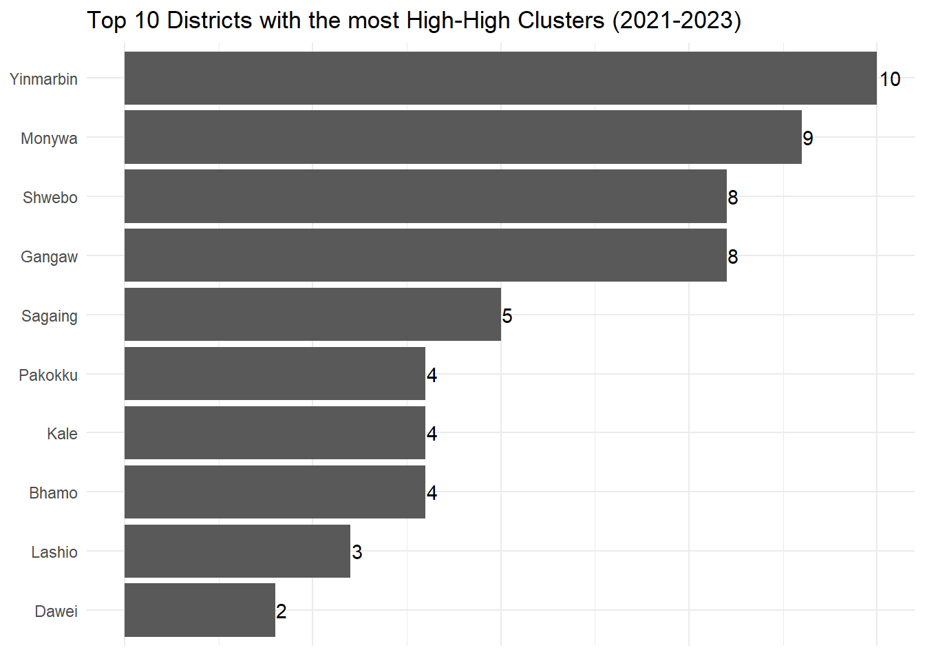
Show the code
lisamap1 <- tm_shape(lisa1) +
  tm_polygons() +
  tm_borders(alpha = 0.5) +
tm_shape(lisa_sig1) +
  tm_fill("mean", style = "pretty", palette = "-RdBu") +
  tm_borders(alpha = 0.4) +
  tm_layout(main.title = "LISA Map for Battles in 2021",
            title = "Quarter 1",
            main.title.size = 0.90,
            legend.height = 0.60,
            legend.width = 5.0,
            legend.outside = FALSE,
            legend.position = c("left", "bottom"))

lisamap2 <- tm_shape(lisa2) +
  tm_polygons() +
  tm_borders(alpha = 0.5) +
tm_shape(lisa_sig2) +
  tm_fill("mean", style = "pretty", palette = "-RdBu") +
  tm_borders(alpha = 0.4) +
  tm_layout(main.title = "LISA Map for Battles in 2021",
            title = "Quarter 2",
            main.title.size = 0.90,
            legend.height = 0.60,
            legend.width = 5.0,
            legend.outside = FALSE,
            legend.position = c("left", "bottom"))

lisamap3 <- tm_shape(lisa3) +
  tm_polygons() +
  tm_borders(alpha = 0.5) +
tm_shape(lisa_sig3) +
  tm_fill("mean", style = "pretty", palette = "-RdBu") +
  tm_borders(alpha = 0.4) +
  tm_layout(main.title = "LISA Map for Battles in 2021",
            title = "Quarter 3",
            main.title.size = 0.90,
            legend.height = 0.60,
            legend.width = 5.0,
            legend.outside = FALSE,
            legend.position = c("left", "bottom"))

lisamap4 <- tm_shape(lisa4) +
  tm_polygons() +
  tm_borders(alpha = 0.5) +
tm_shape(lisa_sig4) +
  tm_fill("mean", style = "pretty", palette = "-RdBu") +
  tm_borders(alpha = 0.4) +
  tm_layout(main.title = "LISA Map for Battles in 2021",
            title = "Quarter 4",
            main.title.size = 0.90,
            legend.height = 0.60,
            legend.width = 5.0,
            legend.outside = FALSE,
            legend.position = c("left", "bottom"))

lisamap5 <- tm_shape(lisa5) +
  tm_polygons() +
  tm_borders(alpha = 0.5) +
tm_shape(lisa_sig5) +
  tm_fill("mean", style = "pretty", palette = "-RdBu") +
  tm_borders(alpha = 0.4) +
  tm_layout(main.title = "LISA Map for Battles in 2022",
            title = "Quarter 1",
            main.title.size = 0.90,
            legend.height = 0.60,
            legend.width = 5.0,
            legend.outside = FALSE,
            legend.position = c("left", "bottom"))

lisamap6 <- tm_shape(lisa6) +
  tm_polygons() +
  tm_borders(alpha = 0.5) +
tm_shape(lisa_sig6) +
  tm_fill("mean", style = "pretty", palette = "-RdBu") +
  tm_borders(alpha = 0.4) +
  tm_layout(main.title = "LISA Map for Battles in 2022",
            title = "Quarter 2",
            main.title.size = 0.90,
            legend.height = 0.60,
            legend.width = 5.0,
            legend.outside = FALSE,
            legend.position = c("left", "bottom"))

lisamap7 <- tm_shape(lisa7) +
  tm_polygons() +
  tm_borders(alpha = 0.5) +
tm_shape(lisa_sig7) +
  tm_fill("mean", style = "pretty", palette = "-RdBu") +
  tm_borders(alpha = 0.4) +
  tm_layout(main.title = "LISA Map for Battles in 2022",
            title = "Quarter 3",
            main.title.size = 0.90,
            legend.height = 0.60,
            legend.width = 5.0,
            legend.outside = FALSE,
            legend.position = c("left", "bottom"))

lisamap8 <- tm_shape(lisa8) +
  tm_polygons() +
  tm_borders(alpha = 0.5) +
tm_shape(lisa_sig8) +
  tm_fill("mean", style = "pretty", palette = "-RdBu") +
  tm_borders(alpha = 0.4) +
  tm_layout(main.title = "LISA Map for Battles in 2022",
            title = "Quarter 4",
            main.title.size = 0.90,
            legend.height = 0.60,
            legend.width = 5.0,
            legend.outside = FALSE,
            legend.position = c("left", "bottom"))

lisamap9 <- tm_shape(lisa9) +
  tm_polygons() +
  tm_borders(alpha = 0.5) +
tm_shape(lisa_sig9) +
  tm_fill("mean", style = "pretty", palette = "-RdBu") +
  tm_borders(alpha = 0.4) +
  tm_layout(main.title = "LISA Map for Battles in 2023",
            title = "Quarter 1",
            main.title.size = 0.90,
            legend.height = 0.60,
            legend.width = 5.0,
            legend.outside = FALSE,
            legend.position = c("left", "bottom"))

lisamap10 <- tm_shape(lisa10) +
  tm_polygons() +
  tm_borders(alpha = 0.5) +
tm_shape(lisa_sig10) +
  tm_fill("mean", style = "pretty", palette = "-RdBu") +
  tm_borders(alpha = 0.4) +
  tm_layout(main.title = "LISA Map for Battles in 2023",
            title = "Quarter 2",
            main.title.size = 0.90,
            legend.height = 0.60,
            legend.width = 5.0,
            legend.outside = FALSE,
            legend.position = c("left", "bottom"))

lisamap11 <- tm_shape(lisa11) +
  tm_polygons() +
  tm_borders(alpha = 0.5) +
tm_shape(lisa_sig11) +
  tm_fill("mean", style = "pretty", palette = "-RdBu") +
  tm_borders(alpha = 0.4) +
  tm_layout(main.title = "LISA Map for Battles in 2023",
            title = "Quarter 3",
            main.title.size = 0.90,
            legend.height = 0.60,
            legend.width = 5.0,
            legend.outside = FALSE,
            legend.position = c("left", "bottom"))

lisamap12 <- tm_shape(lisa12) +
  tm_polygons() +
  tm_borders(alpha = 0.5) +
tm_shape(lisa_sig12) +
  tm_fill("mean", style = "pretty", palette = "-RdBu") +
  tm_borders(alpha = 0.4) +
  tm_layout(main.title = "LISA Map for Battles in 2022",
            title = "Quarter 4",
            main.title.size = 0.90,
            legend.height = 0.60,
            legend.width = 5.0,
            legend.outside = FALSE,
legend.position = c("left", "bottom"))tmap_arrange(lisamap1, lisamap2, lisamap3, lisamap4,
lisamap5, lisamap6, lisamap7, lisamap8,
lisamap9, lisamap10, lisamap11, lisamap12,
ncol=4, nrow=3)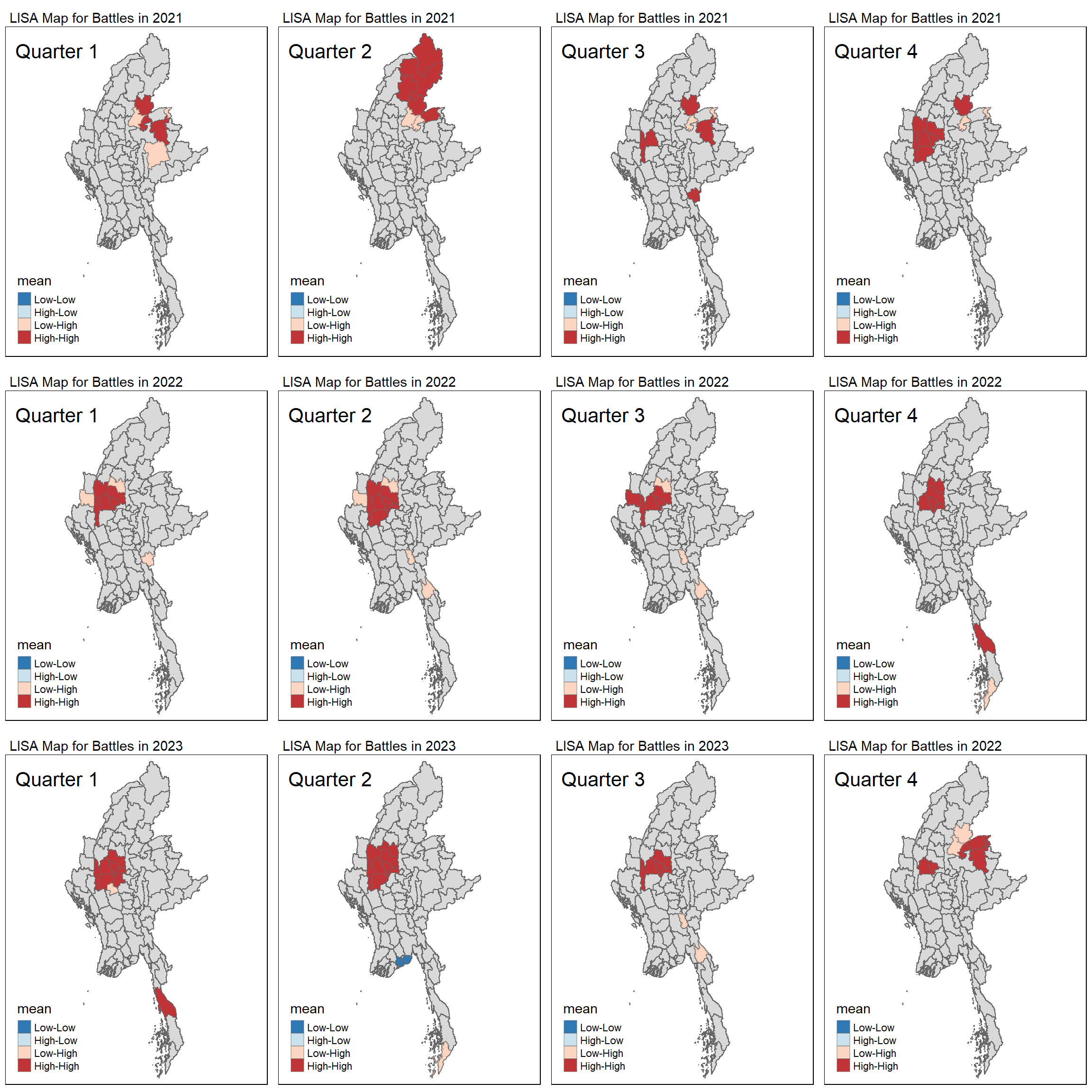
Hot and Cold Spot Analysis (HCSA)
Computing local Gi* statistics
We will need to derive a spatial weight matrix before we can compute local Gi* statistics. Code chunk below will be used to derive a spatial weight matrix by using sfdep functions and tidyverse approach.
Show the code
wm_idw1 <- Battles2021Q1 %>%
  mutate(nb = st_contiguity(geometry),
         wts = st_inverse_distance(nb, geometry,
                                   scale = 1,
                                   alpha = 1),
         .before = 1)

wm_idw2 <- Battles2021Q2 %>%
  mutate(nb = st_contiguity(geometry),
         wts = st_inverse_distance(nb, geometry,
                                   scale = 1,
                                   alpha = 1),
         .before = 1)

wm_idw3 <- Battles2021Q3 %>%
  mutate(nb = st_contiguity(geometry),
         wts = st_inverse_distance(nb, geometry,
                                   scale = 1,
                                   alpha = 1),
         .before = 1)

wm_idw4 <- Battles2021Q4 %>%
  mutate(nb = st_contiguity(geometry),
         wts = st_inverse_distance(nb, geometry,
                                   scale = 1,
                                   alpha = 1),
         .before = 1)

wm_idw5 <- Battles2022Q1 %>%
  mutate(nb = st_contiguity(geometry),
         wts = st_inverse_distance(nb, geometry,
                                   scale = 1,
                                   alpha = 1),
         .before = 1)

wm_idw6 <- Battles2022Q2 %>%
  mutate(nb = st_contiguity(geometry),
         wts = st_inverse_distance(nb, geometry,
                                   scale = 1,
                                   alpha = 1),
         .before = 1)

wm_idw7 <- Battles2022Q3 %>%
  mutate(nb = st_contiguity(geometry),
         wts = st_inverse_distance(nb, geometry,
                                   scale = 1,
                                   alpha = 1),
         .before = 1)

wm_idw8 <- Battles2022Q4 %>%
  mutate(nb = st_contiguity(geometry),
         wts = st_inverse_distance(nb, geometry,
                                   scale = 1,
                                   alpha = 1),
         .before = 1)

wm_idw9 <- Battles2023Q1 %>%
  mutate(nb = st_contiguity(geometry),
         wts = st_inverse_distance(nb, geometry,
                                   scale = 1,
                                   alpha = 1),
         .before = 1)

wm_idw10 <- Battles2023Q2 %>%
  mutate(nb = st_contiguity(geometry),
         wts = st_inverse_distance(nb, geometry,
                                   scale = 1,
                                   alpha = 1),
         .before = 1)

wm_idw11 <- Battles2023Q3 %>%
  mutate(nb = st_contiguity(geometry),
         wts = st_inverse_distance(nb, geometry,
                                   scale = 1,
                                   alpha = 1),
         .before = 1)

wm_idw12 <- Battles2023Q4 %>%
  mutate(nb = st_contiguity(geometry),
         wts = st_inverse_distance(nb, geometry,
                                   scale = 1,
                                   alpha = 1),
         .before = 1)
No of sim = 199
Show the code
HCSA1 <- wm_idw1 %>%
  mutate(local_Gi = local_gstar_perm(
    Incidents, nb, wt, nsim = 199),
         .before = 1) %>%
  unnest(local_Gi)

HCSA2 <- wm_idw2 %>%
  mutate(local_Gi = local_gstar_perm(
    Incidents, nb, wt, nsim = 199),
         .before = 1) %>%
  unnest(local_Gi)

HCSA3 <- wm_idw3 %>%
  mutate(local_Gi = local_gstar_perm(
    Incidents, nb, wt, nsim = 199),
         .before = 1) %>%
  unnest(local_Gi)

HCSA4 <- wm_idw4 %>%
  mutate(local_Gi = local_gstar_perm(
    Incidents, nb, wt, nsim = 199),
         .before = 1) %>%
  unnest(local_Gi)

HCSA5 <- wm_idw5 %>%
  mutate(local_Gi = local_gstar_perm(
    Incidents, nb, wt, nsim = 199),
         .before = 1) %>%
  unnest(local_Gi)

HCSA6 <- wm_idw6 %>%
  mutate(local_Gi = local_gstar_perm(
    Incidents, nb, wt, nsim = 199),
         .before = 1) %>%
  unnest(local_Gi)

HCSA7 <- wm_idw7 %>%
  mutate(local_Gi = local_gstar_perm(
    Incidents, nb, wt, nsim = 199),
         .before = 1) %>%
  unnest(local_Gi)

HCSA8 <- wm_idw8 %>%
  mutate(local_Gi = local_gstar_perm(
    Incidents, nb, wt, nsim = 199),
         .before = 1) %>%
  unnest(local_Gi)

HCSA9 <- wm_idw9 %>%
  mutate(local_Gi = local_gstar_perm(
    Incidents, nb, wt, nsim = 199),
         .before = 1) %>%
  unnest(local_Gi)

HCSA10 <- wm_idw10 %>%
  mutate(local_Gi = local_gstar_perm(
    Incidents, nb, wt, nsim = 199),
         .before = 1) %>%
  unnest(local_Gi)

HCSA11 <- wm_idw11 %>%
  mutate(local_Gi = local_gstar_perm(
    Incidents, nb, wt, nsim = 199),
         .before = 1) %>%
  unnest(local_Gi)

HCSA12 <- wm_idw12 %>%
  mutate(local_Gi = local_gstar_perm(
    Incidents, nb, wt, nsim = 199),
         .before = 1) %>%
  unnest(local_Gi)
Calculating the significant p-vals < 0.05
Show the code
HCSA_sig1 <- HCSA1  %>%
  filter(p_value < 0.05)

HCSA_sig2 <- HCSA2  %>%
  filter(p_value < 0.05)

HCSA_sig3 <- HCSA3  %>%
  filter(p_value < 0.05)

HCSA_sig4 <- HCSA4  %>%
  filter(p_value < 0.05)

HCSA_sig5 <- HCSA5  %>%
  filter(p_value < 0.05)

HCSA_sig6 <- HCSA6  %>%
  filter(p_value < 0.05)

HCSA_sig7 <- HCSA7  %>%
  filter(p_value < 0.05)

HCSA_sig8 <- HCSA8  %>%
  filter(p_value < 0.05)

HCSA_sig9 <- HCSA9  %>%
  filter(p_value < 0.05)

HCSA_sig10 <- HCSA10  %>%
  filter(p_value < 0.05)

HCSA_sig11 <- HCSA11  %>%
  filter(p_value < 0.05)

HCSA_sig12 <- HCSA12  %>%
  filter(p_value < 0.05)
Show the code
HCSA_sig1_1 <-  HCSA_sig1 %>%
  select(cluster, DT, quarter)

HCSA_sig2_1 <-  HCSA_sig2 %>%
  select(cluster, DT, quarter)

HCSA_sig3_1 <-  HCSA_sig3 %>%
  select(cluster, DT, quarter)

HCSA_sig4_1 <-  HCSA_sig4 %>%
  select(cluster, DT, quarter)

HCSA_sig5_1 <-  HCSA_sig5 %>%
  select(cluster, DT, quarter)

HCSA_sig6_1 <-  HCSA_sig6 %>%
  select(cluster, DT, quarter)

HCSA_sig7_1 <-  HCSA_sig7 %>%
  select(cluster, DT, quarter)

HCSA_sig8_1 <-  HCSA_sig8 %>%
  select(cluster, DT, quarter)

HCSA_sig9_1 <-  HCSA_sig9 %>%
  select(cluster, DT, quarter)

HCSA_sig10_1 <-  HCSA_sig10 %>%
  select(cluster, DT, quarter)

HCSA_sig11_1 <-  HCSA_sig11 %>%
  select(cluster, DT, quarter)

HCSA_sig12_1 <-  HCSA_sig12 %>%
  select(cluster, DT, quarter)
Show the code
# Bind the data frames together
combined_df2 <- bind_rows(HCSA_sig1_1, HCSA_sig2_1,
                         HCSA_sig3_1, HCSA_sig4_1,
                         HCSA_sig5_1, HCSA_sig6_1,
                         HCSA_sig7_1, HCSA_sig8_1,
                         HCSA_sig9_1, HCSA_sig10_1,
                         HCSA_sig11_1, HCSA_sig12_1,)
Show the code
quarter_summary_df2 <- combined_df2 %>%
  group_by(DT, cluster) %>%
  summarize(
    Quarters = paste(unique(quarter), collapse = ", "),
    .groups = 'drop'
  )
Show the code
wide_quarter_summary_df2 <- quarter_summary_df2 %>%
  pivot_wider(
    names_from = cluster,
    values_from = Quarters,
    values_fill = list(Quarters = NA)  # Fill with NA where there are no quarters
)print(wide_quarter_summary_df2)Simple feature collection with 28 features and 3 fields
Geometry type: GEOMETRY
Dimension: XY
Bounding box: xmin: 93.09198 ymin: 9.696844 xmax: 99.32485 ymax: 28.54554
Geodetic CRS: WGS 84
# A tibble: 28 × 4
DT geometry Low High
<chr> <GEOMETRY [°]> <chr> <chr>
1 Bawlake POLYGON ((97.52725 19.33779, 97.52732 19.34059, 97.524… 2022… 2021…
2 Bhamo POLYGON ((97.19567 24.90225, 97.1954 24.90408, 97.1909… 2023… 2021…
3 Dawei MULTIPOLYGON (((98.13264 13.53337, 98.13266 13.53345, … <NA> 2022…
4 Gangaw POLYGON ((94.11823 22.76677, 94.11878 22.7686, 94.1152… <NA> 2021…
5 Hakha POLYGON ((93.3483 23.07166, 93.33987 23.07274, 93.3431… 2022… <NA>
6 Hpa-An MULTIPOLYGON (((97.815 16.52402, 97.81483 16.52413, 97… 2022… <NA>
7 Kale POLYGON ((94.17719 23.65037, 94.17714 23.65038, 94.177… <NA> 2021…
8 Kanbalu POLYGON ((95.10246 23.84708, 95.10219 23.84983, 95.103… 2022… 2022…
9 Katha POLYGON ((95.80617 24.95999, 95.80529 24.95822, 95.793… <NA> 2021…
10 Kawthoung MULTIPOLYGON (((98.10929 9.708863, 98.11007 9.711755, … 2022… <NA>
# ℹ 18 more rows# Remove the geometry column to make it a regular data frame
regular_df2 <- st_drop_geometry(wide_quarter_summary_df2)regular_df2 <- regular_df2 %>%
rename("District" = "DT")
kable(regular_df2)| District | Low | High |
|---|---|---|
| Bawlake | 2022Q1, 2022Q2 | 2021Q3 |
| Bhamo | 2023Q4 | 2021Q1, 2021Q2, 2021Q3, 2021Q4 |
| Dawei | NA | 2022Q4, 2023Q1, 2023Q2 |
| Gangaw | NA | 2021Q3, 2021Q4, 2022Q1, 2022Q2, 2022Q3, 2023Q1, 2023Q2, 2023Q3 |
| Hakha | 2022Q1, 2022Q2 | NA |
| Hpa-An | 2022Q1, 2022Q3 | NA |
| Kale | NA | 2021Q4, 2022Q1, 2022Q2, 2023Q2 |
| Kanbalu | 2022Q1, 2022Q2, 2022Q3 | 2022Q4, 2023Q2 |
| Katha | NA | 2021Q2 |
| Kawthoung | 2022Q4, 2023Q1, 2023Q2 | NA |
| Kokang Self-Administered Zone | 2021Q1, 2021Q3, 2021Q4 | 2023Q4 |
| Lashio | NA | 2021Q1, 2021Q3, 2023Q4 |
| Loilen | 2021Q1 | NA |
| Mohnyin | NA | 2021Q2 |
| Mongmit | 2021Q1, 2021Q2, 2023Q4 | NA |
| Monywa | 2021Q3 | 2021Q4, 2022Q1, 2022Q2, 2022Q3, 2022Q4, 2023Q1, 2023Q2, 2023Q3, 2023Q4 |
| Muse | NA | 2021Q2, 2023Q4 |
| Myingyan | NA | 2023Q1 |
| Myitkyina | NA | 2021Q2 |
| Nyaung-U | 2023Q1 | NA |
| Pa Laung Self-Administered Zone | 2021Q2, 2021Q3 | 2021Q1, 2023Q4 |
| Pakokku | NA | 2021Q4, 2022Q2, 2023Q1, 2023Q2 |
| Puta-O | NA | 2021Q2 |
| Pyinoolwin | NA | 2022Q4 |
| Sagaing | NA | 2022Q2, 2022Q3, 2022Q4, 2023Q1, 2023Q2, 2023Q3 |
| Shwebo | NA | 2021Q4, 2022Q1, 2022Q2, 2022Q3, 2022Q4, 2023Q1, 2023Q2, 2023Q3 |
| Yangon (North) | 2023Q2 | NA |
| Yinmarbin | NA | 2021Q4, 2022Q1, 2022Q2, 2022Q3, 2022Q4, 2023Q1, 2023Q2, 2023Q3, 2023Q4 |
summary_df2 <- combined_df2 %>%
  group_by(DT) %>%
  summarize(
    High_Clusters = sum(cluster == "High"),
    Low_Clusters = sum(cluster == "Low"),
    .groups = 'drop'
  )

# Remove the geometry column to make it a regular data frame
regular_df3 <- st_drop_geometry(summary_df2)
top10_high_df <- regular_df3 %>%
arrange(desc(High_Clusters)) %>%
slice_head(n = 10) %>%
rename("District" = "DT")
kable(top10_high_df)| District | High_Clusters | Low_Clusters |
|---|---|---|
| Monywa | 9 | 1 |
| Yinmarbin | 9 | 0 |
| Gangaw | 8 | 0 |
| Shwebo | 8 | 0 |
| Sagaing | 6 | 0 |
| Bhamo | 4 | 1 |
| Kale | 4 | 0 |
| Pakokku | 4 | 0 |
| Dawei | 3 | 0 |
| Lashio | 3 | 0 |
HCSAbar <- ggplot(data = top10_high_df, aes(x = fct_reorder(District, High_Clusters), y = High_Clusters)) +
  geom_bar(stat = "identity") +
  coord_flip() +
  theme_minimal() +
  theme(axis.title.x = element_blank(), axis.title.y = element_blank(),
        axis.text.x = element_blank()) +
  ggtitle("Top 10 Districts with the most High Clusters (2021-2023)") +
  geom_text(aes(label = High_Clusters), hjust = -0.1)

HCSAbar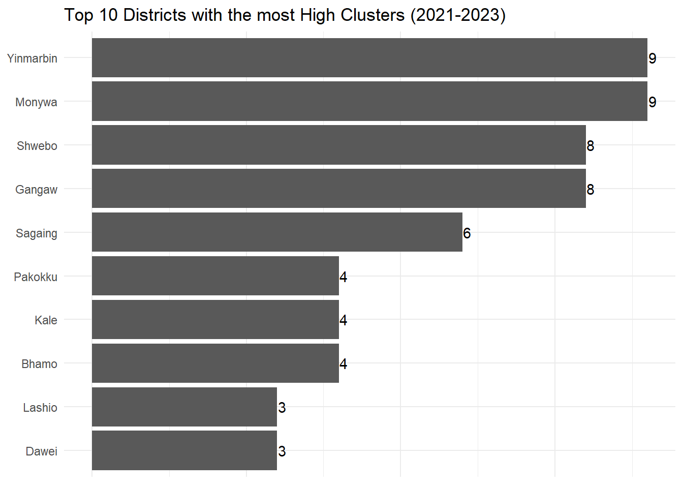
Show the code
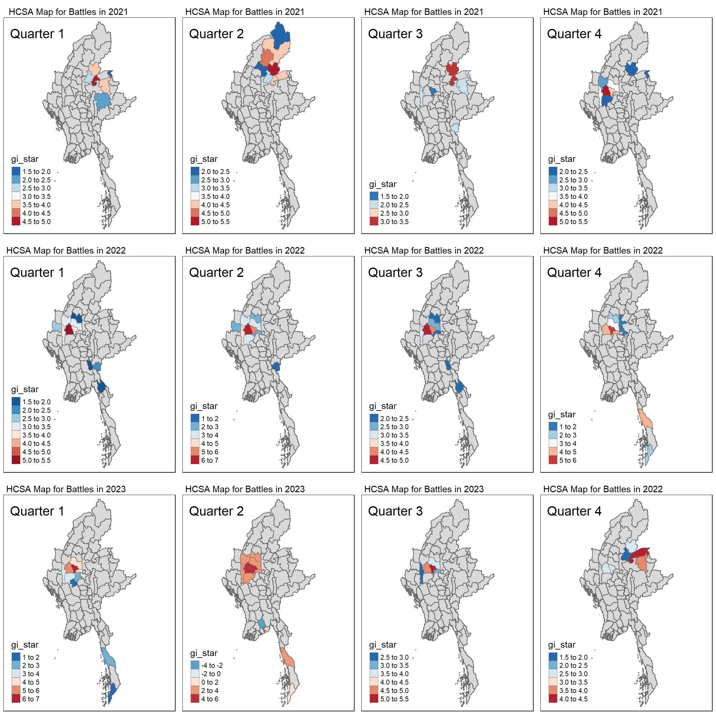
HCSAmap1 <- tm_shape(HCSA1) +
  tm_polygons() +
  tm_borders(alpha = 0.5) +
tm_shape(HCSA_sig1) +
  tm_fill("gi_star", palette = "-RdBu") +
  tm_borders(alpha = 0.4) +
  tm_layout(main.title = " HCSA Map for Battles in 2021",
            title = "Quarter 1",
            main.title.size = 0.90,
            legend.height = 0.60,
            legend.width = 5.0,
            legend.outside = FALSE,
            legend.position = c("left", "bottom"))

HCSAmap2 <- tm_shape(HCSA2) +
  tm_polygons() +
  tm_borders(alpha = 0.5) +
tm_shape(HCSA_sig2) +
  tm_fill("gi_star", palette = "-RdBu") +
  tm_borders(alpha = 0.4) +
  tm_layout(main.title = "HCSA Map for Battles in 2021",
            title = "Quarter 2",
            main.title.size = 0.90,
            legend.height = 0.60,
            legend.width = 5.0,
            legend.outside = FALSE,
            legend.position = c("left", "bottom"))

HCSAmap3 <- tm_shape(HCSA3) +
  tm_polygons() +
  tm_borders(alpha = 0.5) +
tm_shape(HCSA_sig3) +
  tm_fill("gi_star", palette = "-RdBu") +
  tm_borders(alpha = 0.4) +
  tm_layout(main.title = "HCSA Map for Battles in 2021",
            title = "Quarter 3",
            main.title.size = 0.90,
            legend.height = 0.60,
            legend.width = 5.0,
            legend.outside = FALSE,
            legend.position = c("left", "bottom"))

HCSAmap4 <- tm_shape(HCSA4) +
  tm_polygons() +
  tm_borders(alpha = 0.5) +
tm_shape(HCSA_sig4) +
  tm_fill("gi_star", palette = "-RdBu") +
  tm_borders(alpha = 0.4) +
  tm_layout(main.title = "HCSA Map for Battles in 2021",
            title = "Quarter 4",
            main.title.size = 0.90,
            legend.height = 0.60,
            legend.width = 5.0,
            legend.outside = FALSE,
            legend.position = c("left", "bottom"))

HCSAmap5 <- tm_shape(HCSA5) +
  tm_polygons() +
  tm_borders(alpha = 0.5) +
tm_shape(HCSA_sig5) +
  tm_fill("gi_star", palette = "-RdBu") +
  tm_borders(alpha = 0.4) +
  tm_layout(main.title = "HCSA Map for Battles in 2022",
            title = "Quarter 1",
            main.title.size = 0.90,
            legend.height = 0.60,
            legend.width = 5.0,
            legend.outside = FALSE,
            legend.position = c("left", "bottom"))

HCSAmap6 <- tm_shape(HCSA6) +
  tm_polygons() +
  tm_borders(alpha = 0.5) +
tm_shape(HCSA_sig6) +
  tm_fill("gi_star", palette = "-RdBu") +
  tm_borders(alpha = 0.4) +
  tm_layout(main.title = "HCSA Map for Battles in 2022",
            title = "Quarter 2",
            main.title.size = 0.90,
            legend.height = 0.60,
            legend.width = 5.0,
            legend.outside = FALSE,
            legend.position = c("left", "bottom"))

HCSAmap7 <- tm_shape(HCSA7) +
  tm_polygons() +
  tm_borders(alpha = 0.5) +
tm_shape(HCSA_sig7) +
  tm_fill("gi_star", palette = "-RdBu") +
  tm_borders(alpha = 0.4) +
  tm_layout(main.title = "HCSA Map for Battles in 2022",
            title = "Quarter 3",
            main.title.size = 0.90,
            legend.height = 0.60,
            legend.width = 5.0,
            legend.outside = FALSE,
            legend.position = c("left", "bottom"))

HCSAmap8 <- tm_shape(HCSA8) +
  tm_polygons() +
  tm_borders(alpha = 0.5) +
tm_shape(HCSA_sig8) +
  tm_fill("gi_star", palette = "-RdBu") +
  tm_borders(alpha = 0.4) +
  tm_layout(main.title = "HCSA Map for Battles in 2022",
            title = "Quarter 4",
            main.title.size = 0.90,
            legend.height = 0.60,
            legend.width = 5.0,
            legend.outside = FALSE,
            legend.position = c("left", "bottom"))

HCSAmap9 <- tm_shape(HCSA9) +
  tm_polygons() +
  tm_borders(alpha = 0.5) +
tm_shape(HCSA_sig9) +
  tm_fill("gi_star", palette = "-RdBu") +
  tm_borders(alpha = 0.4) +
  tm_layout(main.title = "HCSA Map for Battles in 2023",
            title = "Quarter 1",
            main.title.size = 0.90,
            legend.height = 0.60,
            legend.width = 5.0,
            legend.outside = FALSE,
            legend.position = c("left", "bottom"))

HCSAmap10 <- tm_shape(HCSA10) +
  tm_polygons() +
  tm_borders(alpha = 0.5) +
tm_shape(HCSA_sig10) +
  tm_fill("gi_star", palette = "-RdBu") +
  tm_borders(alpha = 0.4) +
  tm_layout(main.title = "HCSA Map for Battles in 2023",
            title = "Quarter 2",
            main.title.size = 0.90,
            legend.height = 0.60,
            legend.width = 5.0,
            legend.outside = FALSE,
            legend.position = c("left", "bottom"))

HCSAmap11 <- tm_shape(HCSA11) +
  tm_polygons() +
  tm_borders(alpha = 0.5) +
tm_shape(HCSA_sig11) +
  tm_fill("gi_star", palette = "-RdBu") +
  tm_borders(alpha = 0.4) +
  tm_layout(main.title = "HCSA Map for Battles in 2023",
            title = "Quarter 3",
            main.title.size = 0.90,
            legend.height = 0.60,
            legend.width = 5.0,
            legend.outside = FALSE,
            legend.position = c("left", "bottom"))

HCSAmap12 <- tm_shape(HCSA12) +
  tm_polygons() +
  tm_borders(alpha = 0.5) +
tm_shape(HCSA_sig12) +
  tm_fill("gi_star", palette = "-RdBu") +
  tm_borders(alpha = 0.4) +
  tm_layout(main.title = "HCSA Map for Battles in 2022",
            title = "Quarter 4",
            main.title.size = 0.90,
            legend.height = 0.60,
            legend.width = 5.0,
            legend.outside = FALSE,
legend.position = c("left", "bottom"))tmap_arrange(HCSAmap1, HCSAmap2, HCSAmap3, HCSAmap4,
HCSAmap5, HCSAmap6, HCSAmap7, HCSAmap8,
HCSAmap9, HCSAmap10, HCSAmap11, HCSAmap12,
ncol=4, nrow=3)